
As an initial exploration of the collected data, a trial experiment was performed by fitting the raw data to a decision tree model, assessing classification accuracy and feature importance, and visualizing target segmentation.
Data Collection
The predictors used included:
| Property Value Data | Bar/Restaurant Data | Liquor Store Data | Sales Tax Data | Geoanalysis Data |
| Sum of Property Values | Sum, Average, and Standard Deviation of: | Number of Liquor Stores | Number of Businesses | Water |
| Average Property Value | Total Alcohol Sales | Freeway | ||
| Wine Sales | Road | |||
| Beer Sales | Major Road | |||
| Liquor Sales | Parks | |||
| Cover Charge | Urban | |||
| Downtown | ||||
| Civic Building |
Concentric circles were arranged around each target retailer at 5, 10, and 15 mi radii and subdivided into four quadrants (NE, SE, SW, NW), for which each predictor would be calculated and considered. For example, average property value would be calculated for 12 distinct subsections (3 different distances, 4 different quadrants). The sum and average for each concentric circle were also included (e.g., sum of property values at a distance of 5 miles, 10 miles, 15 miles). This brought the feature set to a total of 134 predictors.
The initial feature set included 62 target retailers from Collin County, Dallas County, Denton County and Harris County. The targets included stores that were retail-only, as well as stores that were both wholesale/retail. Classes were determined by total delinquency amount for one delinquency period which covered 12/15/2017 – 12/31/2017. Class distinction by delinquency amounts were as follows: Class 1: >$300k, Class 2: $200k-$300k, Class 3: $100k-$200k, Class 4: <$100k. This division of classes, while seemingly arbitrary, was chosen for ease of interpretation. However, this method did not create optimally equal class sizes.
The 62 x 135 feature set was imported from SQL Server into a Jupyter notebook using pyodbc and converted into a Pandas data frame structure.
Data Preparation
Decision trees bring in the capability to handle a dataset with a high degree of errors and missing values. Due to the limited size of the data set and the relatively few null values present, missing data was treated as a 0 value, rather than removing those records or imputing null values with the mean for that feature.
Typically, machine learning algorithms require several stages of preprocessing and data cleaning. It is necessary when you are solving a system of equations. In decision trees, however, data is simply being compared as the tree is built, so normalization should have no impact on the performance. Therefore, no further preprocessing was performed on the data set for the initial trial run.
Decision Tree Model
Prior to fitting the model, the data was split into train and test subsets using a random 80/20 split, resulting in 49 training examples and 13 test examples.
A single decision tree classifier was fit using the training data using the DecisionTreeClassifier class from scikit-learn’s machine learning library. Fine-tuning of the model was needed to accommodate the set of training features. Rather than using Gini impurity (default metric) as the split criterion, entropy was chosen for its inherent aptness in exploratory analysis. The maximum depth of the tree was set to 3 splits to prevent over-fitting the somewhat scarce training data set.
Results
Accuracy
Prediction accuracy was expectedly low for a first pass of raw data without pre-processing. Out of 7 test samples, only 3 were correctly predicted (42.85% accuracy) using the model above. After adjusting the model to use Gini impurity as a split criterion, the accuracy score dropped to 2 of 7 correctly labeled (28.57% accuracy). In theory, the splitting criteria used should not influence the classification model enough to cause a 14.28% difference in accuracy, which raises concerns about the stability of the given model. Although this first pass is purely a baseline for exploration, no reasonable conclusions can be made until the sample size is increased.
Node Impurity Measures
A visualization of the decision trees for each method of splitting (entropy vs Gini impurity) further demonstrates the necessity of data pre-processing, model selection and increased sample size.
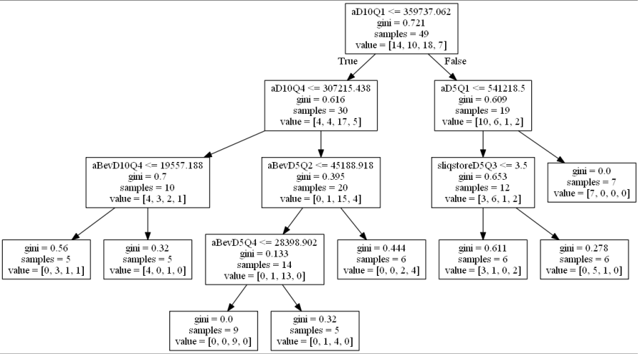
Gini impurity is the probability of a random sample being classified incorrectly if we pick a label according to the distribution in a branch. The Gini index for a node (q) is defined as:
where k is the number of classes (in this case, k=4). It reaches a max value when the samples are equally distributed among all classes, and has a zero value when all samples belong to one class. Ideally the Gini index would reach 0.0 at every terminal leaf in the tree.
The gini index was calculated for each node in the first pass decision tree (see below). The gini impurity reached 0.0 on only two terminal leaves, suggesting the node splits were very impure, and that the rules created by the decision tree were unstable, not easily generalized, and most likely overfit to the the training data.
Entropy, a metric for information gain, measures the impurity of a given node through a log calculation:

where k is the number of classes. If all the samples belong to one class, then entropy is zero. The maximum entropy in the case of k = 4 classes would be 2 (log2(4) = 2). We can see here that the maximum entropy value is 1.916 and largely remains above 1.0, meaning the classes were not properly separated and the rule-based logic of the decision tree was unstable even for the training set.

Feature Importance
The decision tree model found 5-6 features to be the most discriminative, as shown below, the most important being the average property value at distance = 10 mi, quadrant 1. Both methods also used aD5Q1 and a form of total mixed beverage sales at distance 10, quadrant 4 as delineating features. While there is some stability in the features used, they seem fairly arbitrary. Why is the average property value the most important, but only in quadrant 1 at distance 10? Further investigation and due diligence would be necessary to deem this accurate. Otherwise, these results suggest that the decision tree classifier is simply using whatever it can to create rules, whether they are logical or not.


Visualize Data
Scatterplots are commonly used to explore how the feature set segments into separate classes. In order to visualize segmentation of high-dimensional data in a 2D or 3D subspace, some sort of feature selection is required.
Because we do not know the separability of the features without initial exploration of the features involved, creating 3D scatterplots of the raw dataset would provide minimal results at best. It is improbable that any segmentation would occur, as shown below.
Three different principal component analysis techniques were used to reduce data dimensionality:
- PCA – standard PCA is simply a linear dimensionality reduction using singular value decomposition of the dataset to project it to a lower dimensional space. For PCA to have an effect on data, the features must be linearly separable. PCA computes actual principal components out of the feature set which can then be visualized. Here, 3 components were found and mapped into a 3D subspace.
- kPCA – kernel PCA relies on linearly independent feature vectors, so there is no covariance on which to perform eigendecomposition explicitly, as in linear PCA. kPCA, unlike PCA, does not compute the actual principal components themselves, but rather projections of the original dataset onto lower-dimensional components.
A common pitfall in data analytics is the assumption that statistical tools or machine learning techniques, like principal component analyses, will make up for a lack of samples, an overabundance of features, or unclean data. As it has been demonstrated through this trial exploratory run of a decision tree and two types of feature selection, more data is needed, and the data used must be thoroughly examined and cleaned.
After the data set has been properly prepared to be manipulated and analyzed, then more accurate decisions can be made with respect to model selection, feature selection methods, etc. The methodology can continue to evolve as adjustments are made to the approach. Thus is the nature of problem solving with machine learning.
Next Steps
- Sample Size needs to be increased to properly train the decision tree. With only 23 total instances, it is improbable that any amount of data cleaning would allow for the successful segmentation or classification of the data set.
- Thorough data exploration, including univariate and bivariate analysis, missing value treatment, outlier detection, and proper identification of data correlations. Before any type of principal components can be run, it needs to be determined whether or not there is any linear separability of features.
- Continue to make adjustments to the approach and methodology
